Worked example: the Cosmic Eyelash
This page walks through a complete proposal preparation, applying the concepts from the science background to a concrete case. The goal is not just to show you which buttons to click, but to illustrate the reasoning behind each technical choice.
The science case
We want to observe the Cosmic Eyelash (i.e. SMM J2135-0102), a gravitationally lensed starburst galaxy at $z = 2.3$. The goal is to resolve the continuum and molecular gas emission at high angular resolution using ALMA Band 7.
The target observations are:
- CO(9-8) line emission (rest frequency $\nu_\mathrm{rest} = 1036.91\;\mathrm{GHz}$, observed at $\sim 314.2\;\mathrm{GHz}$ at $z = 2.3$)
- Band 7 continuum (around $312\;\mathrm{GHz}$)
Previous observations
We base our planning on two existing datasets:
SMA continuum at 850 μm (Band 7)
- Angular resolution: $\theta_\mathrm{SMA} = 0.2’’$
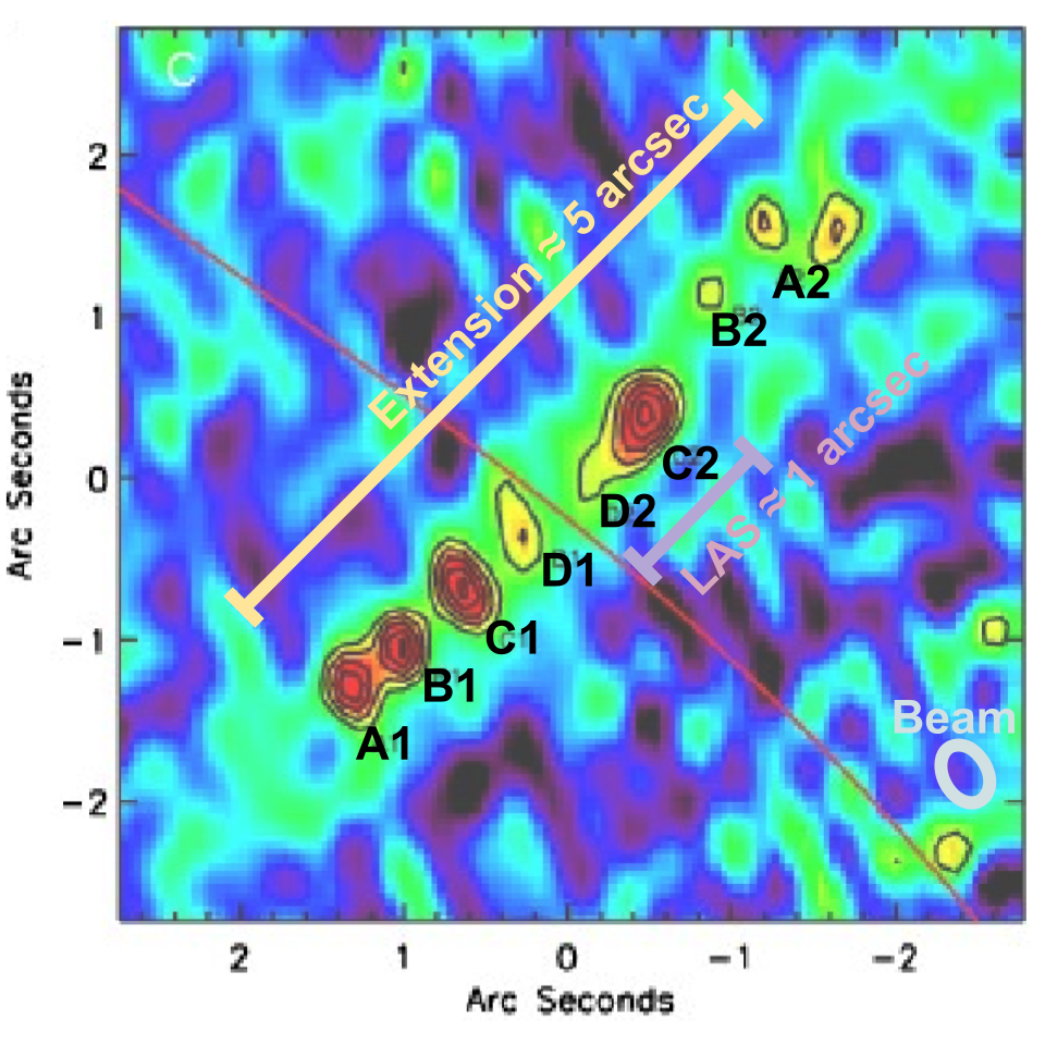
- Source angular extent: $\sim 5’’$
- Multiple resolved components (labelled A1, A2, B1, B2, C1, C2, D1, D2 in the literature)
- Largest angular structure of individual components: $\sim 1’’$
- Total flux density: $S_\mathrm{tot} = 86\;\mathrm{mJy}$
- Faintest component: $\sim 6\;\mathrm{mJy}$ ($3\sigma$ detection)
 |
|---|
| SMA 850 μm continuum image of the Cosmic Eyelash showing the multiple lensed components (Swinbank et al., 2010). |
PdBI CO(3-2) at 104.5 GHz (Band 3)
- Angular resolution: $\theta_\mathrm{PdBI} = 1’’$
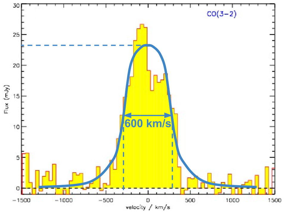
- Gaussian line profile with $\mathrm{FWHM} \approx 600\;\mathrm{km\;s^{-1}}$
- Integrated flux: $F[\mathrm{CO(3\text{-}2)}] = 13.8\;\mathrm{Jy\;km\;s^{-1}}$
- Peak flux density: $F_\mathrm{peak}[\mathrm{CO(3\text{-}2)}] = F[\mathrm{CO(3\text{-}2)}] / \mathrm{FWHM} = 13.8 / 600 \approx 23\;\mathrm{mJy}$
- Source unresolved at $\theta_\mathrm{PdBI} = 1’’$
 |
|---|
| PdBI CO(3-2) spectrum showing the Gaussian-like line profile with FWHM ~600 km/s and peak flux ~23 mJy (Swinbank et al., 2010). |
Choosing the observing band and line
We want CO(9-8), which has a rest frequency of $1036.91\;\mathrm{GHz}$. At $z = 2.3$, the observed frequency is:
\[\nu_\mathrm{obs} = \frac{\nu_\mathrm{rest}}{1 + z} = \frac{1036.91}{3.3} \approx 314.2\;\mathrm{GHz}\]This falls within ALMA Band 7 ($275$–$373\;\mathrm{GHz}$).
You can use Splatalogue to check which CO transitions fall in a given ALMA band at a given redshift. Select the molecule (CO), the band (Band 7), and enter the redshift. At $z = 2.3$ in Band 7, the available CO transitions are $J = 8$–$7$ ($279.3\;\mathrm{GHz}$), $J = 9$–$8$ ($314.2\;\mathrm{GHz}$), and $J = 10$–$9$ ($349.1\;\mathrm{GHz}$).
Angular resolution and largest angular scale
Required angular resolution
The SMA continuum observations resolve the source into multiple components at $\theta_\mathrm{SMA} = 0.2’’$. To resolve these same components with ALMA, we request a similar angular resolution:
\[\theta_\mathrm{ALMA} \approx 0.2''\]In Band 7, ALMA configurations provide angular resolutions ranging from $0.017’’$ to $1.14’’$ for the 12m array, so $0.2’’$ is well within the accessible range.
Largest angular scale
From the SMA image, the individual components have angular sizes of $\sim 1’’$ or less. The total source extent is $\sim 5’’$, but the emission is not uniform — it consists of discrete, compact components. The relevant LAS for our science is the size of the largest individual component, approximately $1’’$.
Do we need ACA?
From the Configuration Information tab in the OT (or from the configuration tables):
- Most extended 12m configuration at $314\;\mathrm{GHz}$: $\mathrm{MRS} \approx 0.17’’$
- Most compact 12m configuration at $314\;\mathrm{GHz}$: $\mathrm{MRS} \approx 9.98’’$
Our estimated LAS of $1’’$ is well below the MRS even for the most compact configuration. ACA is not needed, but the OT already knows. This should be a check for yourself, if ACA is triggered when you did not expect it, maybe you inserted some wrong value somewhere.
If the source had significant smooth emission on scales of several arcseconds (e.g. a diffuse halo around the lensed components), we would need to consider ACA. But based on the SMA image, the emission is concentrated in compact components.
Estimating the CO(9-8) flux
We have not observed CO(9-8) directly. We estimate its flux from the CO(3-2) observations using assumptions about the CO spectral line energy distribution (SLED):
Assumptions:
- CO(9-8) has a Gaussian profile with FWHM similar to CO(3-2): $\mathrm{FWHM} \approx 600\;\mathrm{km\;s^{-1}}$
- The $\mathrm{CO(3\text{-}2)/CO(9\text{-}8)}$ flux ratio is approximately $2.5$ (motivated by models and observations of similar high-redshift starbursts)
This gives:
\[F[\mathrm{CO(9\text{-}8)}] = \frac{F[\mathrm{CO(3\text{-}2)}]}{2.5} = \frac{13.8}{2.5} = 5.52\;\mathrm{Jy\;km\;s^{-1}}\] \[F_\mathrm{peak}[\mathrm{CO(9\text{-}8)}] = \frac{F[\mathrm{CO(9\text{-}8)}]}{\mathrm{FWHM}} = \frac{5.52}{600} \approx 9.2\;\mathrm{mJy/beam}\]These are estimates based on assumed line ratios. The actual CO(9-8) flux could be higher or lower depending on the excitation conditions. State your assumptions clearly in the scientific justification and technical justification of the proposal.
Required sensitivity
This is where the source morphology assumptions become critical. We want $\mathrm{S/N} = 20$ on the CO(9-8) peak. But the required rms depends on what we assume about the source structure at $0.2’’$ resolution (see also Science Background - Peak flux estimation).
Case 1: source unresolved at $\theta_\mathrm{ALMA}$
If the CO(9-8) emission remains unresolved at $\theta_\mathrm{ALMA} = 0.2’’$ (i.e. the emitting region is smaller than $0.2’’$), then the peak flux per beam is the same as the total peak flux:
\[\mathrm{rms} = \frac{F_\mathrm{peak}}{\mathrm{S/N}} = \frac{9.2}{20} \approx 0.5\;\mathrm{mJy/beam}\]Case 2: source resolved into one extended component
If the emission is unresolved at $\theta_\mathrm{PdBI} = 1’’$ but will be resolved by ALMA into a single component of angular size $D \approx \theta_\mathrm{PdBI} = 1’’$ with uniform surface brightness:
\[\mathrm{rms} = \frac{F_\mathrm{peak} \times R}{\mathrm{S/N}} \quad\text{where}\quad R = \left(\frac{\theta_\mathrm{ALMA}}{\theta_\mathrm{PdBI}}\right)^2 = \left(\frac{0.2}{1}\right)^2 = 0.04\] \[\mathrm{rms} = \frac{9.2 \times 0.04}{20} \approx 0.02\;\mathrm{mJy/beam}\]Case 3: source resolved into $N$ components
If the emission is resolved into $N = 5$ components (guided by the SMA continuum morphology), each with angular size $D_\mathrm{cc} = 0.8’’$, with the flux equally and uniformly distributed among them:
\[\mathrm{rms} = \frac{(F_\mathrm{peak}/N) \times R_N}{\mathrm{S/N}} \quad\text{where}\quad R_N = \left(\frac{\theta_\mathrm{ALMA}}{D_\mathrm{cc}}\right)^2 = \left(\frac{0.2}{0.8}\right)^2 = 0.0625\] \[\mathrm{rms} = \frac{(9.2/5) \times 0.0625}{20} \approx 0.006\;\mathrm{mJy/beam}\]Summary of the three cases
| Assumption | rms required |
|---|---|
| Unresolved at $0.2’’$ | $\sim 0.5\;\mathrm{mJy/beam}$ |
| 1 component, $D \approx 1’’$, uniform | $\sim 0.02\;\mathrm{mJy/beam}$ |
| 5 components, $D_\mathrm{cc} \approx 0.8’’$, uniform | $\sim 0.006\;\mathrm{mJy/beam}$ |
The required sensitivity spans nearly two orders of magnitude depending on the assumed morphology. For this source, the SMA continuum data show resolved, compact components, so Case 1 (unresolved) is the most realistic assumption for the individual clumps. We adopt $\mathrm{rms} \approx 0.5\;\mathrm{mJy}$ in a $100\;\mathrm{km\;s^{-1}}$ channel.
Bandwidth used for sensitivity
The CO(9-8) line has an expected $\mathrm{FWHM} \sim 600\;\mathrm{km\;s^{-1}}$. If we want approximately 6 independent velocity channels across the line profile, we need a channel width of $\sim 100\;\mathrm{km\;s^{-1}}$.
The “Bandwidth used for Sensitivity” in the OT should therefore be set to $100\;\mathrm{km\;s^{-1}}$.
This is the velocity resolution at which the requested rms ($0.5\;\mathrm{mJy}$) will be achieved. The native spectral resolution of the correlator will typically be much finer — you average channels in post-processing to reach the desired velocity resolution.
Continuum sensitivity
For the continuum, we use 3 of the 4 basebands (the fourth is allocated to CO(9-8)), giving an aggregate bandwidth of approximately $6\;\mathrm{GHz}$ ($3 \times \sim 2\;\mathrm{GHz}$).
From the SMA data, the faintest continuum component has a flux of $\sim 6\;\mathrm{mJy}$ at $0.2’’$ resolution. If we want to detect it at $\sim 15\sigma$, we need:
\[\mathrm{rms}_\mathrm{cont} \approx \frac{1\;\mathrm{mJy}}{15} \approx 0.07\;\mathrm{mJy/beam}\]With $6\;\mathrm{GHz}$ aggregate bandwidth and the integration time driven by the line sensitivity requirement, the continuum rms achieved is typically well below this threshold. In other words, the continuum is “for free” — the time needed for the line observations already provides more than sufficient continuum sensitivity.
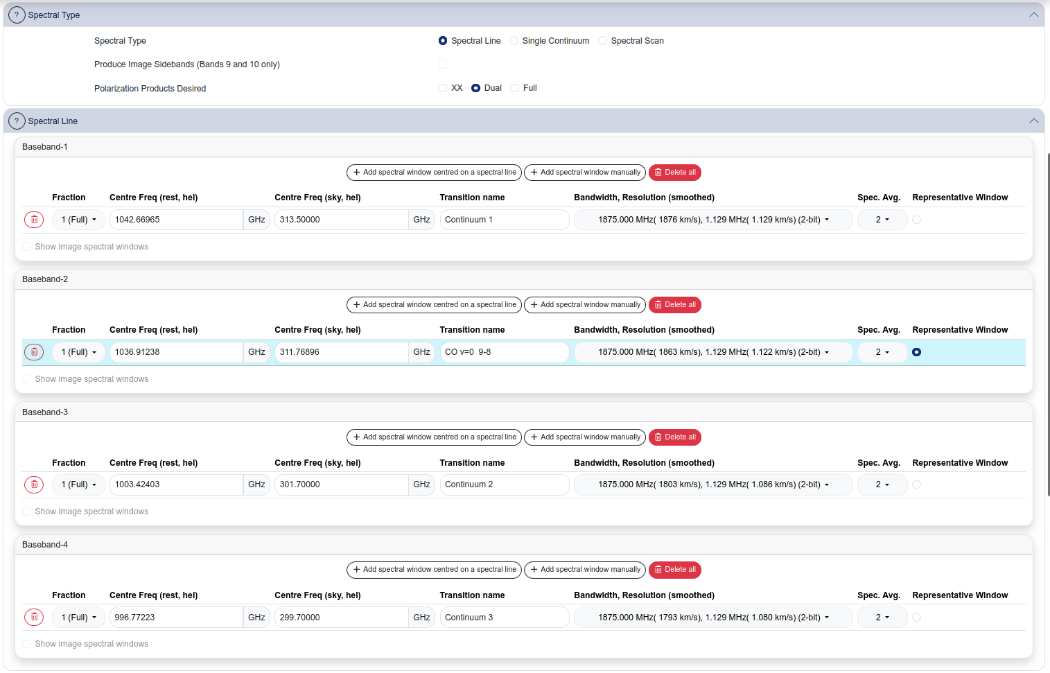
Spectral setup in the OT
The spectral setup for this observation uses Spectral Line type with DUAL polarisation:
- Baseband 1 — continuum, centre frequency $\sim 313.0\;\mathrm{GHz}$ (sky), TDM
- Baseband 2 — CO(9-8), centre frequency $\sim 314.2\;\mathrm{GHz}$ (sky), TDM. This baseband is selected as the Representative Window.
- Baseband 3 — continuum, centre frequency $\sim 301.0\;\mathrm{GHz}$ (sky), TDM
- Baseband 4 — continuum, centre frequency $\sim 302.0\;\mathrm{GHz}$ (sky), TDM
When selected, the requested bands are shown in the frequency visualisation panel at the top of the page: 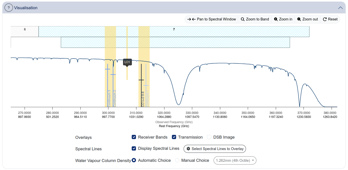
In TDM mode, each baseband provides $\sim 2\;\mathrm{GHz}$ bandwidth with 128 channels, giving $\sim 15.6\;\mathrm{MHz}$ or $\sim 30\;\mathrm{km\;s^{-1}}$ channel width at $314\;\mathrm{GHz}$. In the reality we should also consider Hanning smoothing, which drops the real resolution down to $\sim 31.3\;\mathrm{MHz}$, thus giving us around 60 channels in total. Since we need $100\;\mathrm{km\;s^{-1}}$ channels for the line sensitivity, we are fine.
Control and Performance settings
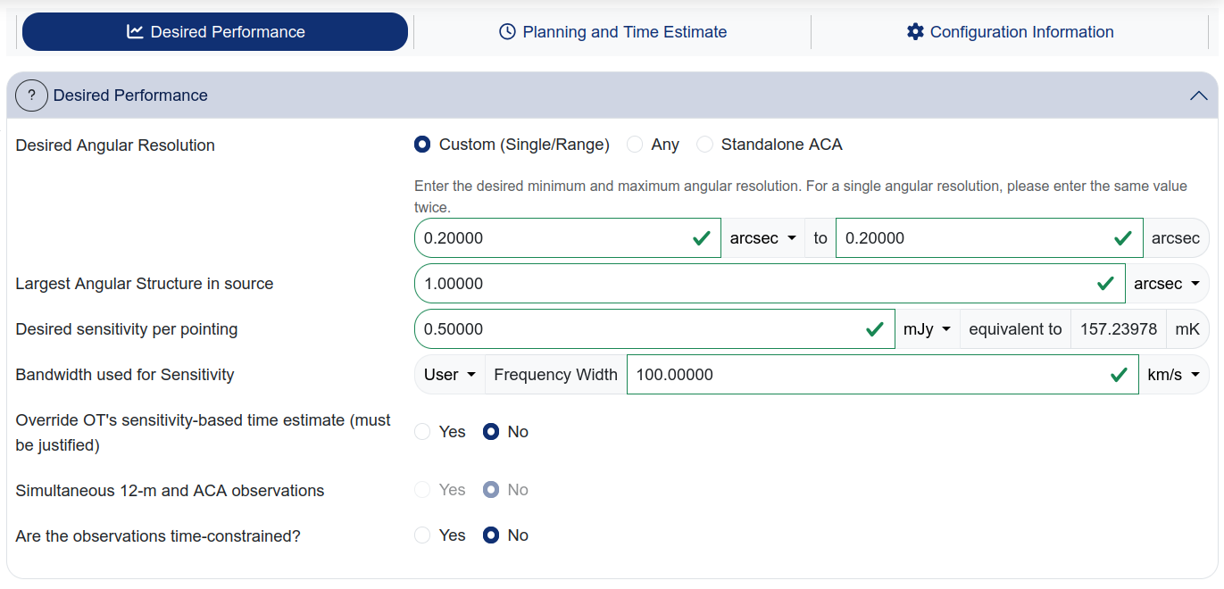
In the Desired Performance sub-tab:
| Parameter | Value |
|---|---|
| Desired Angular Resolution | Custom: $0.2’’$ to $0.2’’$ |
| Largest Angular Structure in source | $1.0’’$ |
| Desired mosaic sensitivity | $0.5\;\mathrm{mJy}$ |
| Bandwidth used for Sensitivity | User, $100\;\mathrm{km\;s^{-1}}$ |
| ACA | No |
| Time-constrained | No |
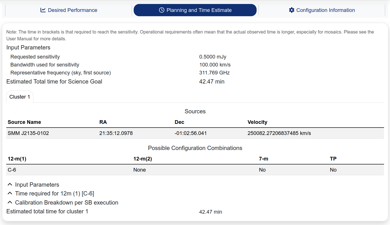
Time estimate
After entering all the parameters, navigate to the Planning and Time Estimate sub-tab to see the estimated observing time.
For this example, the OT gives an estimated total time of approximately $\sim 43$ minutes total, with $\sim 11$ min on source, $\sim 30$ min on calibrators, $\sim 2$ min overheads.
Technical justification
The technical justification for this science goal would cover:
Sensitivity:
We request an rms of $0.5\;\mathrm{mJy}$ in $100\;\mathrm{km\;s^{-1}}$ channels at the representative frequency of $314.2\;\mathrm{GHz}$. This gives $\mathrm{S/N} \approx 20$ on the expected CO(9-8) peak flux of $\sim 9.2\;\mathrm{mJy}$ per beam, assuming the emission is concentrated in compact components unresolved at $0.2’’$ (consistent with the SMA continuum morphology). The aggregate continuum bandwidth of $\sim 6\;\mathrm{GHz}$ gives a continuum rms of $\sim 0.07\;\mathrm{mJy/beam}$, providing $\mathrm{S/N} > 15$ on the faintest continuum component ($\sim 1\;\mathrm{mJy}$).
Imaging:
We request $0.2’’$ angular resolution to match the SMA continuum resolution at 850 μm and resolve the known lensed components. The largest angular structure is $\sim 1’’$ (individual components), well within the MRS of the 12m array. ACA is not needed.
Correlator configuration:
We use TDM with 4 basebands: one centred on CO(9-8) at $314.2\;\mathrm{GHz}$ and three on continuum. The native TDM resolution of 30 km/s is adequate; we will average $\sim 3$ channels to reach $100\;\mathrm{km\;s^{-1}}$ for the line analysis. This gives $\sim 6$ independent velocity channels across the expected CO(9-8) FWHM of $600\;\mathrm{km\;s^{-1}}$.
Entering expected source properties
In the Field setup, the Expected Source Properties should be filled in as:
| Field | Value | Rationale |
|---|---|---|
| Peak Continuum Flux Density per Synthesized Beam | $0.006\;\mathrm{Jy}$ ($6\;\mathrm{mJy}$) | Brightest component from SMA at similar resolution |
| Peak Line Flux Density per Synthesized Beam | $0.0092\;\mathrm{Jy}$ ($9.2\;\mathrm{mJy}$) | Estimated CO(9-8) peak flux (Case 1: unresolved) |
| Line Width | $600\;\mathrm{km\;s^{-1}}$ | From CO(3-2) FWHM |
The OT uses these values to compute S/N estimates displayed in the Technical Justification summary. Make sure they are consistent with the sensitivity you requested — if they are not, the S/N displayed will look wrong and reviewers may notice the inconsistency.